Discussion on Characteristics and Resistance of Automotive Data Cables
What is characteristic impedance
The first indicator requirement for automotive data cables is characteristic impedance. What does this characteristic impedance mean?
Before discussing characteristic impedance, we first need to determine a concept that signals move forward step by step in transmission lines, and the establishment of electromagnetic fields also requires a process. Signals do not propagate from the transmitting end to the receiving end at once.
Each step of forward transmission of the signal will encounter specific capacitance and inductance parameters. Here, we introduce two new variables: "Unit length capacitance C" and "Unit length inductance L".
Characteristic impedance is not a fundamental concept, but a concept applied to transmission lines. In high-speed application scenarios, signal transmission lines can no longer be regarded as ideal wires, and some parasitic parameters on the transmission line, such as parasitic resistance, parasitic capacitance, and parasitic inductance, cannot be ignored. Characteristic impedance is the composite parameter of these parameters in a comprehensive transmission line scenario.
The transmission line per unit length can be equivalent to the following model (as shown in Figure 1):
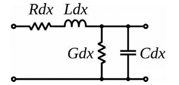
Figure 1 Equivalent Model of Transmission Line
Each step of the signal encounters C and L, and the characteristic impedance at this point is defined as (as shown in Figure 2a). The theoretically accurate characteristic impedance is a frequency dependent quantity. In practical applications, the resistance part of the transmission line, that is, the part that dissipates energy, can often be ignored, that is, the R and G in the above equation are 0, which is approximately a lossless transmission line. For lossless transmission lines, the impedance expression can be expressed as (as shown in Figure 2b):
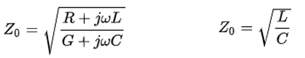
Figure 2 Definition formula of characteristic impedance
The Influence of Characteristic Impedance on Transmission Lines
Characteristic impedance is one of the very important parameters of automotive data cables, and excellent performance cannot be achieved without precise control of impedance. And what we usually call impedance control is to make the transmission line as uniform as possible and reduce reflection, which controls the characteristic impedance.
From the above introduction, it can be seen that the concept of characteristic impedance is based on two or more conductors, so it is necessary to have a good and complete reference plane as the reflux path. We need to avoid the reference plane being cut and cross segmented, which may cause impedance discontinuity and reflection (as shown in Figure 3).
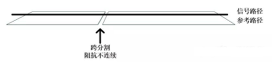
Figure 3 Schematic diagram of signal transmission path
This is like riding a bike on the road, the flatter the road, the faster you ride; If there are small pits on the road, it will be very bumpy and the speed will decrease; So for high-speed signals, good impedance control is crucial (as shown in Figure 4).
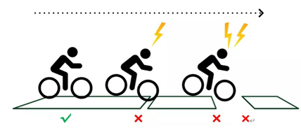
Figure 4 Schematic diagram of uneven impedance
How to test characteristic impedance
In application scenarios such as research and development/design verification, production testing, and quality management, automotive data cables require testing of the product's characteristic impedance. Therefore, a fast, accurate, and standard testing plan can undoubtedly greatly improve testing efficiency.
There are three ways to test characteristic impedance:
1) Measuring impedance using TDR method
Time domain reflectometer (TDR) technology emerged as early as the 1960s. This technology includes generating a time step voltage that propagates along the transmission line. Use an oscilloscope to detect reflections from impedance, measure the ratio of input voltage to reflected voltage, and calculate discontinuous impedance (as shown in Figure 5).
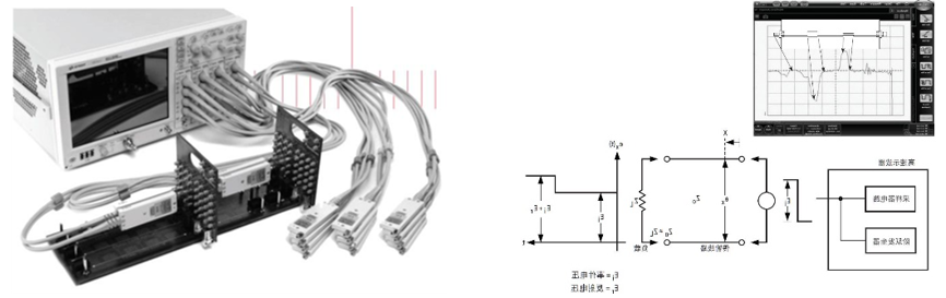
Figure 5 TDR testing equipment and schematic diagram
2) Measuring input impedance using a network analyzer
The network analyzer measures the input impedance on the test port (as shown in Figure 6). Usually, this is not the characteristic impedance of the cable. If the electrical length of the cable is very long, the input impedance is the characteristic impedance of the cable.
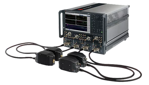
Figure 6 Network Analyzer Test Equipment
3) Using an LCR meter to measure impedance
The so-called "open circuit short circuit" method can be used to measure the low-frequency characteristic impedance (as shown in Figure 7). Measure open circuit and short circuit impedances on the longest cable that can still be considered as a lumped component, typically 1/10 wavelength cable. The square root of the product of two measurement results is the characteristic impedance. The disadvantage of this technology is its low accuracy. Open circuit and short circuit measurements may exceed the reasonable accuracy of the network analyzer. A better method is to use a network analyzer to measure open circuit and short circuit impedances, which can measure a wide impedance range due to the use of current voltage technology.
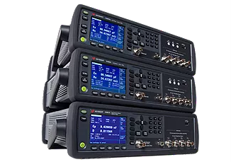
Figure 7 LCR Table Test Equipment
Common characteristic impedance
Various impedance cables are often seen in automotive data cables, including 50 Ω, 75 Ω, 90 Ω, 100 Ω, 120 Ω, etc. The various application scenarios are as follows:
1) The impedance control of the video signal line is 75 Ω.
2) The differential impedance of the USB signal line is 90 Ω.
3) The differential impedance of the Ethernet differential signal line is 100 Ω.
4) The differential impedance of RS422, RS485, and CAN differential signals is 120 Ω
How are these impedance control values determined? Let's choose a 50 Ω characteristic impedance of a coaxial line and a differential impedance of 100 Ω of a twisted pair for an introduction.
① 50 Ω impedance of coaxial line
The selection of 50 Ω as the high-frequency characteristic impedance matching for the coaxial line is based on a comprehensive consideration of power capacity, breakdown resistance voltage, and attenuation. As shown in the figure below, the insertion loss is the smallest, approximately 77 Ω. On the other hand, if the relationship curve between maximum power transmission and characteristic impedance is plotted, the maximum power is approximately 30 Ω.
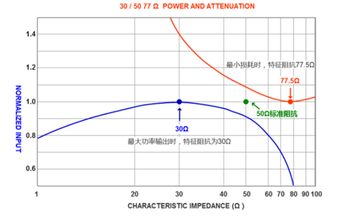
Figure 8 Schematic diagram of 50 Ω impedance
When the maximum power is transmitted, the characteristic impedance value is 30 Ω, while the theoretical minimum attenuation (loss) characteristic impedance is 77.5 Ω. Find a balance point between the transmission power and minimum attenuation values, and select an impedance value of 50 Ω for the transmission line (as shown in Figure 8).
On the other hand, when minimum loss is required in longer coaxial cables (such as cables or satellite TV) and there is no high demand for power transmission, cables and connectors with an impedance of 75 Ω are used in these systems.
② Differential line 100 Ω impedance
When matching at a single end, the impedance is 50 Ω. We have already understood why the differential line is 100 Ω? How to understand this matter?
As shown in Figure 9, for the differential line, we separately parallel a characteristic impedance of Z (assuming 50 Ω) to ground for each transmission line.
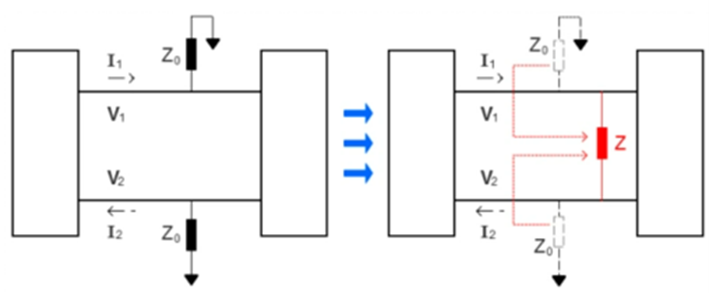
Figure 9 Schematic diagram of 100 Ω impedance
The figure actually shows quite intuitively:
Because: I1=- I2
So: in fact, there is no current passing through the ground to these two Zs, which means they can be combined into a whole, as shown in the red part on the right of the figure, with a size of 2Z, which is why the differential impedance is 100 Ω.
In fact, if the distance between these two transmission lines is too close, there is coupling between them, and because of this coupling, the impedance of each line is not Z. The specific reasoning process will not be elaborated here. We assume that the coupling coefficient is k, so the actual impedance value should be: Z=2Z (1-k).